Course tutorials and video lectures
1. Field spectroscopy : principles and approaches
This lecture will introduce the fundamental principle underlying spectroscopy, is that: a) when light interacts with any media there is a photon energy level and flux density change; b) the light measured by the spectrometer will contain information from: the light source; the atmosphere through which the light has passed; and surfaces or media with which it has interacted. Therefore, light can be used as an ‘information’ carrier. From this information it may, just may, be possible to infer or estimate some properties of the media (atmosphere and/or surface) with which it has interacted if information of the light source is known. So in field spectroscopy it is the energy level, indicated by wavelength, and photon flux density per unit time (radiant flux), often in relation to some standard reference providing information of the light source, that is measured. Attempts can then made to relate the photon flux density per wavelength interval to physical properties of the media and to spectral measurements made by other investigators separated by space and time.
We will then go on to discuss terminology used to describe spectroscopic illumination an viewing geometry definitions and angular dependencies. Then a number of field measurement configurations and practical approaches will be introduced and their limitations discussed. Click on the slide below and then click on the ‘full screen’ icon to run a video of the lecture.
2. Measurement uncertainties
There are errors and uncertainties associated with all physical measurement. Optical remote sensing and field spectroscopy are no different. This second lecture introduces the sources of some of these errors and uncertainties both those associated with instruments use and field measurement methods. The concepts of: measurand; measurement; uncertainties and the geostatistical term ‘support’ are introduced and discussed. For in-depth discussion on metrological terms and method to quantify and report uncertainties readers should refer to “Joint Committee for Guides in Metrology (2008). Evaluation of measurement data; Guide to the expression of uncertainty in measurement. Joint Committee for Guides in Metrology (ISO), 1st edn” and to further understand ‘support’ see Atkinson, P., and Tate, N., (2000) Professional Geographer, 52(4), p 607–623. Click on the slide below and then click on the ‘full screen’ icon to run a video of the lecture.
3. Hyperspectral imaging
This lecture will make the case for hyperspectral imaging and contrast it with multispectral imaging. Hyperspectral imaging from airborne platforms such as the Twin Otter or the Dornier aircraft owned by NERC will be introduced and the additional uncertainties associated with these measurements and platforms will be discussed. Hyperspectral imaging from space-based platforms will also be introduced.
We are now considering making hyperspectral measurements simultaneously over multiple supports. This is in contrast to field spectroscopy measurements, presented in the two previous lectures, where a single hyperspectral measurement is integrated over a single support and further measurements are taken sequentially as required. The measurements in this case are made by a hyperspectral imaging spectrometer which is able to collect multiple measurements in a single row across an Earth surface area. These measurements can then be represented as contiguous pixels perpendicular to the aircraft’s direction of travel. Hyperspectral imagers are normally of a ‘pushbroom’ design and as the aircraft moves forward additional rows of measurements are made. As the imager has an Inertial Measurement Unit (IMU) and a differential GPS, the geographical location and the orientation of the row of measurements is recorded so that an image of the Earth surface covered can be created by orthorectification in post processing. The errors and uncertainties inherent with these imaging instruments and measurement platforms will also be introduced.
4. Flight planning and calibration and validation (cal/val)
This presentation highlights issues related to the planning for the collection of remotely sensed airborne data and issues related to the collection of calibration and validation data. Key considerations for flight planning are when, where and the altitude and flight direction of any data acquisitions. These extend into an evaluation of manual and integrated flight planning. Cal/val touches on the difference between calibration and validation, what is vicarious calibration and a brief consideration of the discrepancies of scale when comparing data collected from field, airborne and satellite systems. The presentation culminates with the combination of these two topics with respect to the collection of calibration and validation data from the study site at the Barrax experimental farm (Albacete) during field studies associated with this lecture.
5. Field sampling strategies
This presentation led into a tutorial that addressed (i) Support, (ii) the Sampling Scheme and (iii) measurements necessary for appropriate statistics and statistical robustness) relating to optimal field sampling for model parameterisation and cal/val of airborne and satellite measurements from field measurements from the Barrax experimental farm, Alcacete.
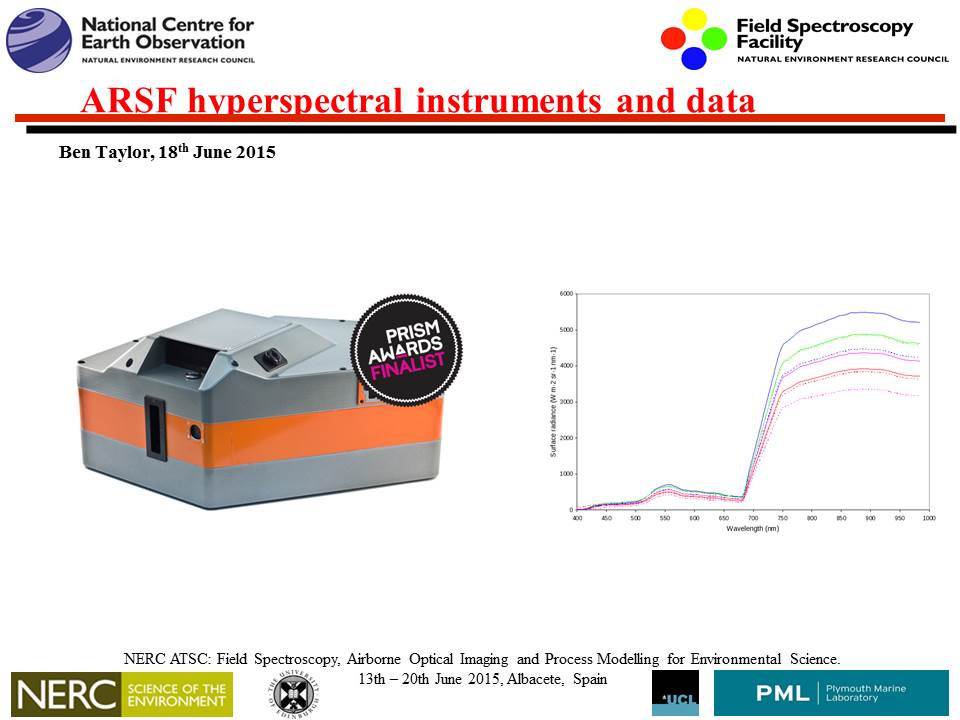
6. NERC Airborne Survey Facility hyperspectral instruments
This presentation briefly introduces the spectral imagers that have been used by the ARSF and goes on to provide more detail about the current and recent hyperspectral instrument suite, including Visible, Near Infra-Red, Short-Wave Infra-Red and Thermal Infra-Red imagers
7. Tour of the aircraft at the NERC Airborne Survey Facility
This virtual tour of one of the NERC research aircraft demonstrates the suite of remotely sensed instruments typically from by NERC for airborne remote sensing; these instruments include LiDAR, imaging spectrometers and a digital camera.
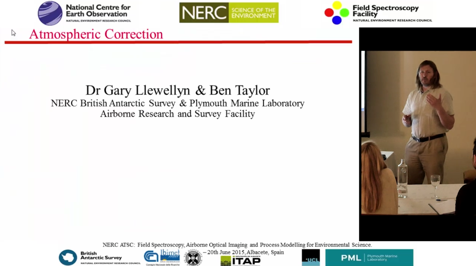
8. Atmospheric correction of hyperspectral images
This demonstration starts with a brief consideration of the attenuation of a remotely sensed signal from a ground target presented by the atmosphere and suggests several methods by which it may be corrected. Although empirical and image-based methods are introduced the main demonstration uses a popular covariance matrix & radiative transfer modelled method, Atcor4.
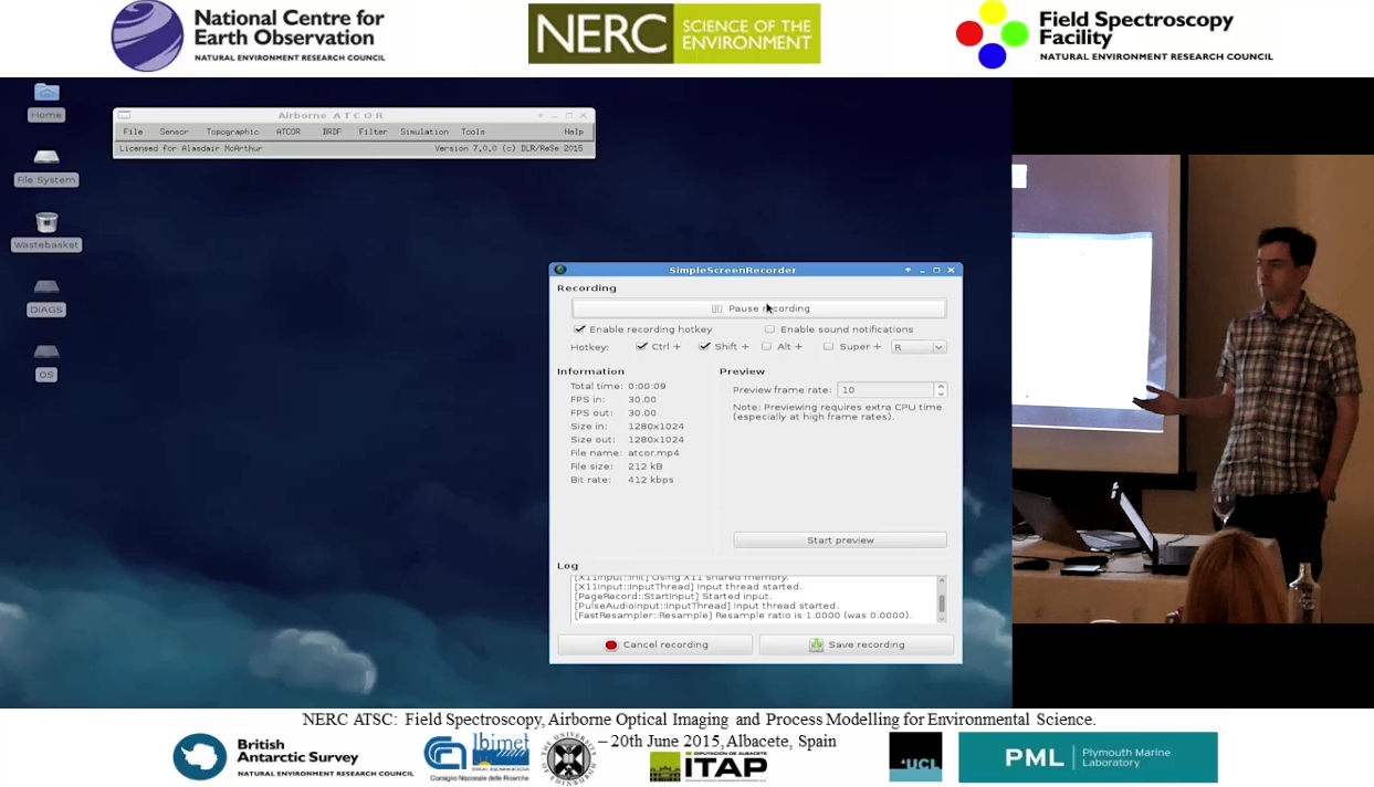
9. Using atmospheric correction models: ATCOR4
This lecture provides a basic introduction to use of the ATCOR program for atmospheric correction of airborne spectral data. It provides an overview of some of the basic functions in ATCOR and how to use them, along with the data requirement to run the program. Note that it does NOT describe how to do atmospheric correction accurately, only how to run ATCOR itself and get basic output.
10. Hyperspectral data processing and use of APL
This lecture describes how to process ARSF hyperspectral sensor data using the Airborne Processing Library (APL) software suite. It describes why the data need to be processed, runs through the different processing stages that are part of the suite and leads into the hyperspectral processing practical session.
11. Introduction to radiative transfer modelling
The first part of the lecture introduces the motivation behind radiative transfer (RT) theory. RT allows one to describe the processes that govern the fate of a photon interacting with a medium, for example a photon from the sun that is absorbed or scattered by the atmosphere or by a canopy. This provides a description of how the reflectance data that you acquire is collected. For vegetation canopies, RT theory indicates that the optical properties of leaves (in turn governed by pigment concentrations and internal leaf structure) and the geometrical disposition of leaves within a canopy are intimately convolved in the reflectance spectra that you might measure, so both aspects need to be understood in order to fully learn about parameters linked to leaf physiology or to canopy structure. Link to presentation slides.
The second part of the lecture introduces some concepts of leaf RT modelling, with a particular focus on the PROSPECT leaf model (a leaf reflectance and transmittance model that has been widely used). Link to presentation slides.
12. Radiative transfer of leaves and canopies
This lecture covers a basic introduction to canopy RT modelling. Once the properties of leaves have been determined, we can develop a model of how a photon would be scattered or absorbed by a medium made up of a uniform distribution of leaves with a particular reflectance and transmittance. In this talk, we will look at how the first order scattering can be calculated, and include some comments on how the higher order terms can be estimated. Link to presentation slides.
13. Inferring the characteristics of the surface from optical data
A typical application of RT models is inferring the state of the land surface (e.g. estimate LAI or canopy chlorophyll concentration from measured reflectances). In this lecture, we cover some of the aspects of inversion. Link to presentation slides.
14. The course field data set contains:
Apogee chlorophyll meter estimates of leaf chlorophyll content; Delta-T Sunscan estimates of LAI; Field spectroscopic measurements of maize and wheat leaf and canopy and reference panel radiant flux for conversion to reflectance; Nadir and BRDF field spectroscopic measurements of invariant and natural vicarious calibration targets for the atmospheric correction and/or validation of atmospheric correction of hyperspectral airborne images; Sky hemispherical photos and global irradiance data.
Group A carried out field spectroscopy cal/val measurements using SVC HR-1024i #2003 and Microtops #7346.
Group B carried leaf chlorophyll estimates using an Apogee Chlorophyll meter and LAI estimates using a Delta-T sunscan.
Group C carried out canopy reflectance and leaf reflectance and transmission spectroscopic measurement using ASD FieldSpecPro #6239.
Global irradiance was recorded by the host Fernando de la Cruz Tercero, ITAP- Instituto Técnico Agronómico Provincial (ITAP) at Las Tiesas using an Ocean Optics HR4000 #HR4C2516 with standard Ocean Optics RCR. In addition, supplementary canopy and leaf measurements of wheat were made on 18/06/2015.
There are ReadMe.txt files for each individual data set providing information on location and measurement descriptions.
These data (180mb) can be down loaded from here.
Questions regarding individual group data sets should be addressed to the relevant persons listed in each data set’s ReadMe.txt
15. Field spectroscopy measurement post-processing.
The first step in post-processing field spectrometric measurements is to calculate relative reflectance (reflectance is a computed term. Radiance, and possibly exitance, is what is measured from a surface by a field spectrometer). So relative reflectance is target surface radiance relative to some standard, normally a Spectralon, or similar reference panel, or ‘white-plate’. See here.
Relative reflectance R rel (λ) as a function of wavelength λ is defined as the ratio of the target radiance spectrum L(λ) to the corresponding relative reference spectrum E rel (λ). E rel (λ) should be a radiance measurement of a reference standard taken simultaneously or near-simultaneously (i.e. under the same illumination conditions as the target radiance)
R rel (λ) = L(λ)/Erel (λ)
The second step if to determine ‘absolute’ reflectance so that these results can be compared to the results of others made using other Spectralon panels or reference standards. These standards should be calibrated to that the difference between their reflectance per wavelength interval and 100% reflectance per wavelength interval is known (R panel cal. coeffs. (λ)). Calibration coefficients should be provided with reference standards used and should be current as the reflectance of these standards changes over time and with use. Panels can be cleaned (see Spectralon® Care and Handling Guidelines. ) but should be sent to a dedicated spectroscopy calibration laboratory of back to the manufacturer for recalibration after cleaning.
R abs (λ) = L(λ) / (E(λ)/ R panel cal. coeffs.(λ))
A Matlab Spectroscopy Toolbox and User Guide, developed by Dr I. Robinson and Dr A, Mac Arthur, with a wide range of field spectroscopy post-processing function is available from Matlab Central here or a range of Excel templates, developed by Mr C. MacLellan, to calculate reflectance is available from here.
The FSF panel calibration coefficients can also be downloaded from here. Please take care to select the coefficients for the panel used.
14. The NERC/BAS ARF campaign data set.
The processed image data (Level 1b and Level 2 atmospherically corrected only – first look) collected using the ARF FENIX can be downloaded from here. Note CEDA will provide ‘open’ access, however you will need to register as a CEDA user. See Centre for Environmental Data Analysis registration page here. A tutorial on empirical line correction, using these images and data collected during the NERC ATSC at Barrax during 2015, has been developed by the NERC ARF Data Analysis Node at PML and can be accessed here